A while ago I followed a course in Machine Learning on Coursera. In this course I did some exercises in R, which is a language suitable for statistical computing and data analysis. Because I am a Java software engineer, I wanted to try to do it in Java.

There are various libraries and platforms that support Machine Learning with Java and since I have some experience with Apache Spark, which supports Java, I decided to use that.

So in this blog I will give an introduction to Machine Learning, followed by a short introduction to Apache Spark before I combine these two in an actual example.

An introduction to Machine Learning

Machine Learning is generally about creating algorithms for learning and predicting based on data.

Applications for Machine Learning for example are spam filtering, optical character recognition (OCR), recommendation engines (think suggestions what to watch next based on user preferences, previous watched films, etcetera), prediction of risks for insurance companies and fraud detection based on transactions for banks.

Basically the goal is to create a prediction algorithm (also called a model) based on a set of data. There are three kinds of predictions:

• Supervised prediction, when you have a dataset labelled with the desired outputs, for example used in spam filtering or image recognition like OCR.
• Unsupervised prediction, when you don’t have the desired outputs, for example to cluster data based on features, like analysing purchase patterns of customers.
• Forecasting, when you use historical data for predicting the future, for example when you want to predict stock market trends based on historical transactions.

The principle of all three kinds of predictions is the same, although the splitting of data and use of algorithms may vary.

When you know what to predict you need a set of matching input data. For example, you need a set of bank transactions to predict fraud in bank transactions. From this set of input data a set of characteristics (features) is extracted, which can be used for the prediction.

The input data is split in a training set and a test set. The training set is used to create a model with one or more statistical data algorithms and the test set is used for evaluation of the model. When you have a model you are satisfied with, you can use the model for predicting with unlabelled data.

Feature extraction

Not all input data is suitable for predictions. Besides needing corresponding data, you also need features that contain relevant information for the prediction.

Using all data can lead to overfitting of the algorithm, meaning that it performs well on the training set but poorly on the test set, because the model is tailored to the training set. So typically features are selected that describe the data with sufficient accuracy.

Feature extraction can be done manually or can be done automatically. Manual feature extraction is usually difficult, time-consuming and requires expert knowledge. Automatic feature extraction can be done by dimension reduction techniques such as Principal Component Analysis, which converts a set of possibly correlated values into a set of linear uncorrelated variables called principal components.

This reduced set of features is called a feature vector.

Splitting of datasets

To train the model you need data. But you don’t want to use the same data to evaluate the model, so you have to split the dataset in a training set for training the model and a test set for evaluating the model.

If you use the same set for both training and evaluating you might not detect errors in the model because the model is too tailored to the training set (overfitting).

There are various ways to split the dataset. Some of the most common are the following techniques:

• Random subsampling: this method splits the dataset randomly into training and test data. This can be repeated a number of times and the results are then averaged in a single prediction model.
• K-Fold: this method breaks up the dataset into k equal sized subsets and uses k-1 subsets as training data and 1 subset as test data. This is repeated k times. The results are then averaged to produce a single prediction model.
• Leave-one-out: this method takes one sample from the dataset as test data to evaluate the model and use the rest for training data to build the model. This is repeated for every sample of the dataset and the results are averaged to a single prediction model.

The bigger the dataset, the bigger the chance of accurate results. The goal is to create a model with a high accuracy (precision) and low fault tolerance (called Out of sample Error).

For forecasting the dataset is split up into time slices.

Training the model

After we have determined the features and split the dataset in a training and test set we start training the model for prediction.

There are various algorithms for machine learning, some of them are:

• Regression: regression analysis is used to examine the relationship between one dependent variable and independent variables. Usually it is used for continuous or linear models.
• Decision trees: decision trees are used in classification predictions. A model is created which will predict the outcome based on the input variables and guide them through the decisions in the tree.
• Bootstrap aggregating: also called bagging is a variance reduction technique that is used to improve the predictive performance of decision trees by generating a bootstrap sample from the training set and calculating the predictions a number of times. Combining the results either by averaging or majority vote.
• Random Forest: random forest is an extension of bootstrapping. For each bootstrap sample it creates multiple decision trees and averages the result.
• Boosting: boosting is a bias reduction technique and typically improves the performance of a single tree model by combining weak features (only slightly correlated) into a stronger one.

These algorithms can also be combined together (called an ensemble) to create a better prediction algorithm. A disadvantage of these ensemble algorithms is that they tend to be slower.

Evaluate the model

When we have created a model using an algorithm with a training set, we can evaluate the model with the test set. Usually we want to check the accuracy of the model.

An introduction to Apache Spark

Apache Spark is an open source data processing framework for performing Big Data analytics on a distributed computing cluster. It supports a variety of datasets that are diverse in nature (text, graphs, etc.) as well as diverse data sources (like batch data or real time streaming data).

It is written in Scala and runs on the Java Virtual Machine and it supports programming languages like Java, Scala, Python and R. It runs standalone, in a cluster, on Hadoop, Mesos or in the cloud.

It even runs in Docker containers.

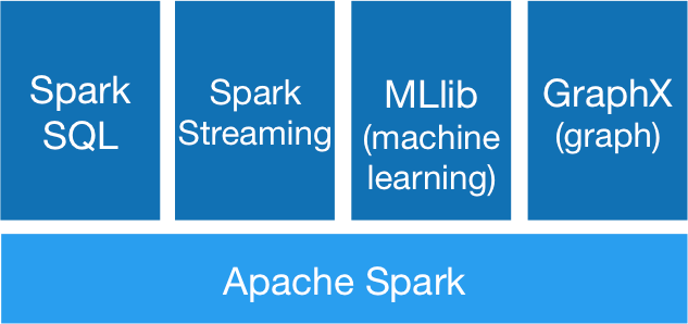
It consists of four modules on top of the Spark engine which can be combined to do complex data analysis. These modules are:

• Spark SQL: Spark SQL is used for working with structured data. It allows you to access any data source the same way. You can either use SQL or the DataFrame API to connect to a variety of data sources, joining data across these sources. Also connections to Spark are possible using JDBC or ODBC.
• Spark Streaming: Streaming is a scalable fault-tolerant streaming API which lets you write stream jobs the same way as batch jobs.
• Spark MLlib: MLlib is a scalable machine learning library containing a lot of machine learning algorithms and utilities.
• Spark GraphX: GraphX is Apache Spark’s API for graphs and graph-parallel computation. It supports ETL, exploratory analysis and iterative graph computing. You can view the same data as graphs or collections and transform and join graphs, or write custom graph algorithms.

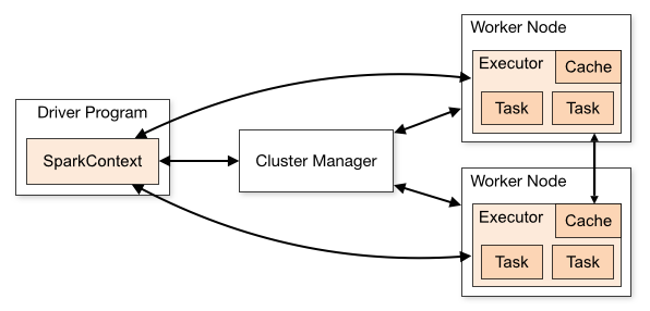
A Spark cluster typically consists of a Cluster Manager (master) and Worker nodes. Spark applications run as independent processes on this cluster, coordinated by the SparkContext object in the main (driver) program. A Spark application is submitted to the master and then connects to Spark.

Once connected, Spark acquires executors on nodes in the cluster, which are processes that run computations and store data for your application. Next, it sends the application code to the executors. Finally, SparkContext sends tasks to the executors to run.

A cluster (both master and worker nodes) can be monitored using a web-based user interface, which is accessed through the master.

Note: Since Apache Spark 2.0 the SparkContext object is encapsulated within a SparkSession object, which also provides a unified access to Sparks data source API’s like SQL, DataFrame, DataSet, etc.

Running a Spark Machine Learning application on Apache Spark

So, now it is time to create a Machine Learning application and run it on Apache Spark!

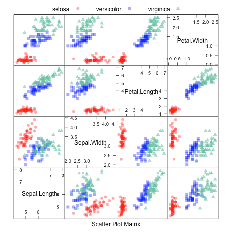
For this example I use the classic Iris dataset from the UCI Machine Learning Repository. It contains three Iris flower species with 50 samples each. One flower species is linearly separable from the other two, but the other two are not linearly separable from each other.

The columns in this dataset are:

• Id
• SepalLengthCm
• SepalWidthCm
• PetalLengthCm
• PetalWidthCm
• Species

Where SepalLengthCm, SepalWidthCm, PetalLengthCm and PetalWidthCm are the features and Species is the resulting class. Species in this case are Iris-setosa, Iris-versicolor and Iris-virginica.

The first 5 rows of the dataset are (in csv-format):

Id,SepalLengthCm,SepalWidthCm,PetalLengthCm,PetalWidthCm,Species
1,5.1,3.5,1.4,0.2,Iris-setosa
2,4.9,3.0,1.4,0.2,Iris-setosa
3,4.7,3.2,1.3,0.2,Iris-setosa
4,4.6,3.1,1.5,0.2,Iris-setosa
5,5.0,3.6,1.4,0.2,Iris-setosa

It is beyond the scope of this article to show how to plot a scatter plot matrix with Apache Spark GraphX, so I have included the scatter plot matrix of my R exercise to show the relations between the four features.

So let’s start with the creation of our Spark application. For ease of use, everything will be done in the main method of a Java class.

To summarize the steps to be taken, we need to read the data from the dataset, identify the features and split the dataset into a training and test set. Then we create a model with a Machine Learning algorithm (in this case I have used Random Forest) and use this model to predict the outcome of the test set.

First we create a SparkSession object and read the dataset (in csv-format) from disk.

// initialise Spark session
SparkSession sparkSession = SparkSession.builder().appName("SparkIris").getOrCreate();

// load dataset, which has a header at the first row
Dataset rawData = sparkSession.read().option("header", "true").csv(PATH);

Then we create a feature vector containing all the features and split the dataset in a training and test set. The training set is 70% of the dataset and the test set 30%. We use a seed for the randomSplit so the results can be reproduced when we run this application again.

// identify the feature colunms
String[] inputColumns = {"SepalLengthCm", "SepalWidthCm", "PetalLengthCm", "PetalWidthCm"};
VectorAssembler assembler = new VectorAssembler().setInputCols(inputColumns).setOutputCol("features");
Dataset featureSet = assembler.transform(rawData);

// split data random in trainingset (70%) and testset (30%)
long seed = 5043;
Dataset[] trainingAndTestSet = featureSet.randomSplit(new double[]{0.7, 0.3}, seed);
Dataset trainingSet = trainingAndTestSet[0];
Dataset testSet = trainingAndTestSet[1];

Next we can offer the training set to the Random Forest algorithm to produce a model.

// train the algorithm based on a Random Forest Classification Algorithm with default values
RandomForestClassifier randomForestClassifier = new RandomForestClassifier().setSeed(seed);
RandomForestClassificationModel model = randomForestClassifier.fit(trainingSet);

Now we can test and evaluate the accuracy of the model against the test set.

// test the model against the test set       
Dataset predictions = model.transform(testSet);

// evaluate the model
MulticlassClassificationEvaluator evaluator = new MulticlassClassificationEvaluator()
        .setLabelCol("label")
        .setPredictionCol("prediction")
        .setMetricName("accuracy");

System.out.println("accuracy: " + evaluator.evaluate(predictions));

The result of this program is:

accuracy: 0.9393939393939394

Even without tuning the Random Forest algorithm, we get an accuracy of almost 94%. This means that only 3 of the 45 test samples are predicted wrong. Not bad for a first try.

To see the predictions of the test data we can use

predictions.select("id", "label", "prediction").show();

Now that we have a model we are satisfied with, we are ready to start predicting a new Iris dataset without labels for Iris species.

🌼 🙂

PS In this article I have given a short overview of Machine Learning and Apache Spark with an example of how to use the Apache Spark Machine Learning library. Note that the source code presented in this article is simplified because I have left out showing intermediate results and some transformations which are necessary for the Random Forest algorithm (like converting the Species classification values to discrete numbers).

PPS The complete source code with (references to) instructions how to run this on an Apache Spark cluster (standalone or Docker based) can be found on my GitHub.